1.1. Fourier Series¶

Note

You can run and modify code as you read along this page by clicking the launch button then Live Code button on the top of this page. Alternatively, the Binder button redirects you to another page to run cells with a traditional Jupyter Notebook interface.

1.1.1. Definition¶

For simplicity, we will restrict ourselves to functions \(f(x)\) defined on the domain \(x \in [0, 1]\). Then the \(N\)th partial sum of the Fourier series of \(f(x)\) is

(1.1)¶\[ f_N(x) = \frac{a_0}{2} + \sum_{n=1}^N \left[ a_n \cos\left(2\pi nx\right) + b_n \sin\left(2\pi nx\right) \right] \]

where the so-called Fourier coefficients are

(1.2)¶\[\begin{split} a_n = 2 \int_{0}^{1} f(x) \cos\left(2\pi nx\right), \\ b_n = 2 \int_{0}^{1} f(x) \sin\left(2\pi nx\right). \end{split}\]

When \(N\) is small, \(f_N(x)\) is usually a poor approximation of \(f(x)\) because \(f_1(x)\) consists of only one frequency. As \(N\) increases the approximation improves, reaching exact convergence everywhere when \(N = \infty\).

1.1.2. Example: \(f(x) = x\)¶

The Fourier coefficients, (1.2), are

(1.3)¶\[\begin{align} a_n &= 2 \int_{0}^{1} x \cos\left(2\pi nx\right), \\ b_n &= 2 \int_{0}^{1} x \sin\left(2\pi nx\right). \end{align}\]

It’s not too hard to calculate these integrals via integration by parts, but it’s even easier to use sympy:

import sympy as sp
sp.init_printing(use_latex='mathjax')

x, a_n, b_n = sp.symbols('x a_n b_n', real=True)
n = sp.symbols('n', integer=True, nonnegative=True)
f, u = x, 2*sp.pi*n*x

sp.integrate(2*f*sp.cos(u), (x, 0, 1))

\[\begin{split}\displaystyle \begin{cases} 0 & \text{for}\: n \neq 0 \\1 & \text{otherwise} \end{cases}\end{split}\]

sp.Eq(a_n, sp.integrate(2*f*sp.cos(u), (x, 0, 1)))

\[\begin{split}\displaystyle a_{n} = \begin{cases} 0 & \text{for}\: n \neq 0 \\1 & \text{otherwise} \end{cases}\end{split}\]

sp.Eq(b_n, sp.integrate(2*f*sp.sin(u), (x, 0, 1)))

\[\begin{split}\displaystyle b_{n} = \begin{cases} - \frac{1}{\pi n} & \text{for}\: n \neq 0 \\0 & \text{otherwise} \end{cases}\end{split}\]

Direct substitution into (1.1) yields Fourier series

(1.4)¶\[ f_N(x) = \frac{1}{2} - \sum_{n=1}^N \frac{\sin\left(2\pi nx\right)}{\pi n}. \]

1.1.3. Visualization¶

Let’s plot (1.4) for various \(N\):

import matplotlib.pyplot as plt
import numpy as np

def get_fourier_sums(xs, N):
    fourier_sums = np.zeros(len(xs)) + .5
    for n in range(1, N+1):
        fourier_sums -= np.sin(2*np.pi*n*xs) / (np.pi*n)
    return fourier_sums

dx = .01
xs = np.arange(0+dx, 1, dx)
fig, ax = plt.subplots()
ax.set(xlabel='$x$', ylabel='$f_N(x)$', title='Fourier series for $f(x)=x$')
ax.plot(xs, get_fourier_sums(xs, 1), label='$N=1$')
ax.plot(xs, get_fourier_sums(xs, 10), label='$N=10$')
ax.plot(xs, get_fourier_sums(xs, 100), label='$N=100$')
ax.legend();

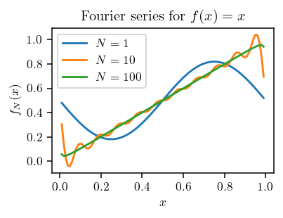
Clearly \(N = 1\) is a poor approximation because it consists of a single sinusoidal term. \(N = 10\) captures the linear portion but has visible oscillations. \(N = 100\) appears much smoother and matches \(f(x) = x\) closely except at the boundaries. The boundary disagreement is because the Fourier series is periodic by nature and thus approximates a sawtooth wave when the domain is extended:

xs = np.arange(0+dx, 3, dx)
fig, ax = plt.subplots()
ax.set(xlabel='$x$', ylabel='$f_N(x)$', title='Extended Fourier series for $f(x)=x$')
ax.plot(xs, get_fourier_sums(xs, 100));

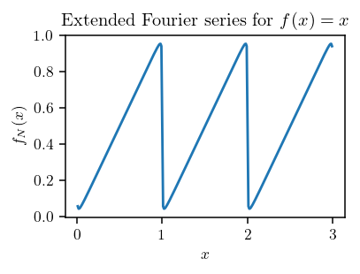
Due to discontinuities at integer values of \(x\), the Fourier series actually takes the midpoint value \(\frac{1}{2}\).

Proof

When \(x\) is an integer, \(nx\) is also an integer and thus \(2\pi n x\) is an integer multiple of \(2\pi\). It follows that \(\sin(2\pi n x) = 0\) for all \(n\). Looking at the calculated Fourier series, (1.4), it follows that \(f_N(x) = \frac{1}{2}\). \(\blacksquare\)

1.1.4. Interactive Animation¶

The Fourier series plot for various \(N\) in § Visualization is helpful in distingushing different qualitative behaviors, but difficult to see how \(f_N(x)\) changes with \(N\). Of course, we could repeatedly make plots tuning \(N\) by hand, but interactive slider plots do that much better, for example:

import ipywidgets

@ipywidgets.interact(N=ipywidgets.IntSlider(min=1, max=100, step=1))
def fourier_slider(N):
    dx = .01
    xs = np.arange(0+dx, 1, dx)
    fig, ax = plt.subplots()
    ax.set(xlabel='$x$', ylabel='$f_N(x)$', title='Fourier series for $f(x)=x$')
    ax.plot(xs, get_fourier_sums(xs, N), label=f'$N={N}$')
    ax.plot(xs, xs, '--', label='$f(x) = x$')
    ax.legend()

If you’re reading this on the online webpage, dragging the slider has no effect on the plot. To see live updating, you must click on the launch button at the top of the page and launch with Binder. Thebe currently does not work due to lack of additional javascript required from ipywidgets.

Exercise

Compute the Fourier series \(f_N(x)\) of the function \(f(x) = \lvert x - \frac{1}{2}\rvert\) over the interval \(x \in [0, 1]\). Plot \(f_N(x)\) for three values of \(N\) with different quailtative behavior. Finally, make an interactive slider plot of \(f_N(x)\), letting \(N\) be an adjustable parameter.

Hint

In sympy, \(\lvert x - \frac{1}{2}\rvert\) can be represented symbolically as

sympy.Abs(x - sp.Rational(1/2))

Solution

def get_fourier_sums(xs, N):
    fourier_sums = np.zeros(len(xs)) + .25
    for n in range(1, N+1, 2):  # Even terms are zero
        fourier_sums += np.cos(2*np.pi*n*xs) * 2 / (np.pi*n)**2
    return fourier_sums

@ipywidgets.interact(N=ipywidgets.IntSlider(min=1, max=50, step=1))
def fourier_slider(N):
    dx = .01
    xs = np.arange(0+dx, 1, dx)
    fig, ax = plt.subplots()
    ax.set(xlabel='$x$', ylabel='$f_N(x)$', title='Fourier series of $|x - \\frac{1}{2}|$')
    ax.plot(xs, get_fourier_sums(xs, N), label=f'$N={N}$')
    ax.plot(xs, np.abs(xs - .5), '--', label='$|x - \\frac{1}{2}|$')
    ax.legend()

# Your code goes here.

Jupyter Book Demo

1.1. Fourier Series¶

1.1.1. Definition¶

1.1.2. Example: \(f(x) = x\)¶

1.1.3. Visualization¶

1.1.4. Interactive Animation¶